RapidFEM

Open-source Maxwell FEM in Rust. Frequency and time domain behind one Python API.

RapidFEM is an electromagnetic FEM solver written in Rust, distributed as a Python package. Two backends sit behind one geometry / material / physics API: a frequency-domain solver (Nedelec curl-conforming edge elements of first and second order, mixable within one mesh, complex-symmetric sparse linear algebra) and a time-domain DGTD solver (nodal discontinuous Galerkin with Krylov/ETD exponential time integration and model order reduction). Geometry is non-dimensionalized before assembly, so sub-micron RFIC passives and metre-scale antennas use the same numerical path.

import numpy as np
import rapidfem as rf

g = rf.Geometry(maxh=rf.lambda_maxh(f_max=12e9))
air = g.box(22.86e-3, 10.16e-3, 30e-3,
            position=(-11.43e-3, -5.08e-3, 0), material=rf.Air())

rf.RectWaveguidePort(air.faces.min(axis="z"))
rf.RectWaveguidePort(air.faces.max(axis="z"))
rf.PEC(*air.faces.unassigned)
g.mesh()

prob = rf.Problem(g)
result = prob.sweep(np.linspace(8e9, 12e9, 21))
# the same Problem also drives eigenmode solves and far-field patterns

Two backends, one API

The frequency-domain solver came first: solve each frequency directly, get S-parameters, fields and modes out of it. The DGTD backend was added for what the discontinuous Galerkin operator makes possible. It is element-local, which is the shape of computation a GPU wants, and it is where operator-level model order reduction can be tried. It also never forms a factorization, so a mesh that is too large to factor is still solvable.

Both backends read the same geometry, the same materials and the same ports, so choosing between them is a keyword rather than a second model.

The workflow

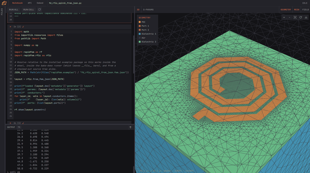
Distribution is a plain pip install: pip install rapidfem ships ahead-of-time compiled wheels for Windows, Linux, and macOS. No Rust toolchain, no vendor install, no license server. External CAD comes in as STEP, IGES, or BREP and lands in the same geometry kernel as the primitives, so imported parts take booleans, transforms, and physics exactly like a g.box(); STL is healed into a meshable solid. For RFIC work, process stacks and GDS layouts become 3D geometry via rapidfem.rfic: the octagonal spiral above is a layout description loaded straight into the solver, meshed through its dielectric stack, with the S-parameters of the run below the code that produced it. Validated end-to-end examples ship with the package, from microstrips and coupled lines through iris and stepped-impedance filters to patch, Vivaldi, and inverted-F antennas, pyramidal horns, dielectric resonators, and on-chip passives.

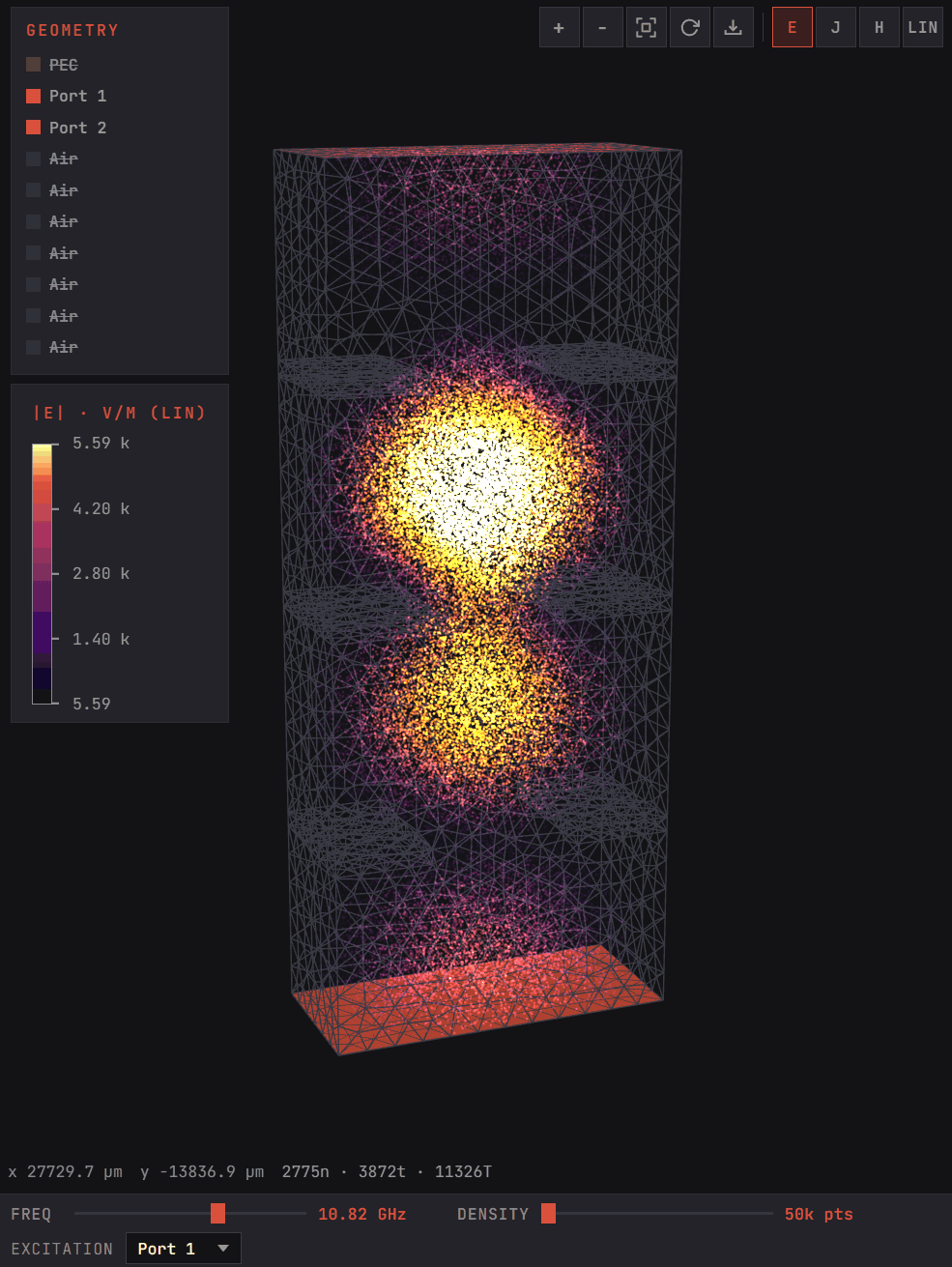
The UI is a notebook rather than a CAD program. Building a CAD front end is its own multi-year project, and the setups people write here are code anyway. What was missing was the part CAD does well: seeing the thing. So the notebook keeps the code workflow and puts interactive geometry, mesh and field renderers next to it, which makes a simulation inspectable at every stage instead of a black box behind a job queue. The renderer itself comes largely from RapidPassives , extended for tetrahedral meshes and mesh display. Above: an iris-coupled waveguide filter driven from port 1 at 10.82 GHz, the field rendered as a point cloud over the tetrahedral mesh, so the two coupled cavities and the evanescent irises between them are visible in the same view as the geometry that produced them.

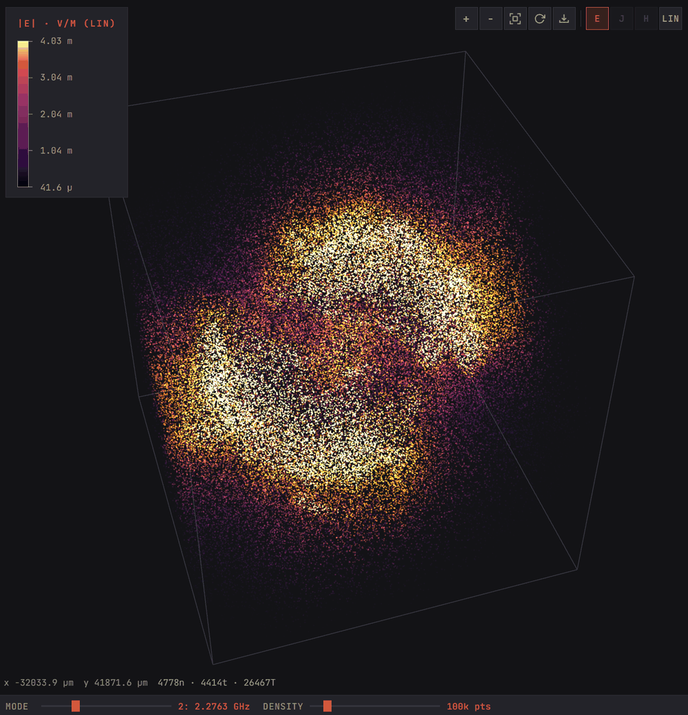
The same renderer draws eigenmodes: here the second mode of a dielectric resonator at 2.2763 GHz. An eigenmode solve has no excitation, so the field plot is what identifies which mode came out.

History

RapidFEM began in April 2026 as a Rust port of emerge, by Robert Fennis. The DGTD time-domain backend came on top of that, built because I wanted to experiment with running the operator on a GPU and with operator-level model order reduction, and because large meshes need a solver that does not have to hold a factorization.

Since then it has been completely reimplemented: its own kernels, first- and second-order basis functions, and the assembly rebuilt to mix the two orders in one mesh. Mixed order is what the RFIC path needs. Fine structures drive the element count up until the degrees of freedom explode, and being able to spend second-order elements only where the field asks for them, while the already dense regions stay first order, is what keeps such a system small enough to solve at all.

The notebook UI and the RFIC path came with the reimplementation. Meshing and linear algebra currently come from gmsh and PARDISO; moving onto RapidMesh and RSLAB is where the stack is heading.